Running on the Desktop
OpenCL Background
SeaRay uses a Python wrapper for OpenCL, called PyOpenCL, to accelerate certain computations. OpenCL is designed to interface with arbitrary computing devices, especially multi-core CPU and general purpose GPU (GPGPU) devices. The user can specify a particular device to use, or allow SeaRay to select one. If there are errors related to memory or floating point precision you can try a different device.
Running the Tests
You should test the installation by running the unit tests:
python -m pytest
If any of the tests fail consider checking out a different version.
Running a Ray Example
Activate your virtual environment (see Generic SeaRay Installation)
Pick some example from
raysroot/examples/eikonal/.For definiteness, let us use
raysroot/examples/eikonal/parabola.pyOpen a terminal window and navigate to
raysrootpython rays.py listThe above command lists the hardware acceleration platforms and devices available on your system. A device may be available only within a given platform. If there is more than one platform, choose the one you would like to use, and pick out some unique part of its name, such as
cuda. Case does not matter. Similarly, if there is more than one device, choose some unique part of its name, such astitanpython rays.py run file=examples/eikonal/parabola.py platform=cuda device=titanThis copies the
parabola.pyexample file to theraysrootdirectory asinputs.pyand runs the calculation. If you do not specify a file, SeaRay will use whateverinputs.pyis inraysroot. It is best practice to never directly editinputs.py.When the run is finished, you should have several output files in
raysroot/out. The output files are simply pickled numpy arrays.Let us plot the results using the SeaRay plotter. The plotter is not interactive, but allows for a fairly high degree of control using command line options. You can get a help screen by executing
python plotter.pywith no arguments.python plotter.py out/test o3dYou should see a 3D rendering of the ray orbits reflecting off an off-axis parabola, as in Fig. 1 below (assuming
matplotlibenvironment). When you are done looking close the plot window.python plotter.py out/test det=1,2/0,0/0.1This should produce an image of the radiation intensity at the focal point, as in Fig. 2 below.
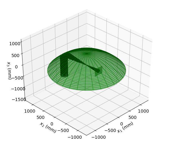
Fig. 1 — ray orbits from parabolic mirror example
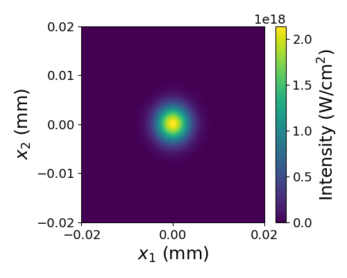
Fig. 2 — Intensity at best focus
Running a Wave Example
Activate your virtual environment (see Generic SeaRay Installation)
Run the example case
raysroot/examples/paraxial/air-fil.pyfollowing the same general procedure as above.Wave runs typically take longer, although this one is fairly quick. You should see some text based progress indicators as the wave propagation is calculated. The time stepper is adaptive, so varying amounts of work may be done between diagnostic planes.
Run the Jupyter notebook
viewer.ipynbusing your favorite notebook interface (Chrome, VS Code, etc.).For this example you should not need to change the source code. Generally, if output files are saved under a different location you have to change the value of
base_diagnostic. Note also that as of this writing, the normalizing length is hard coded in the notebook.Run the notebook (e.g. select
Run Allfrom theCellmenu). Advance the z-slider to observe the pulse evolution.
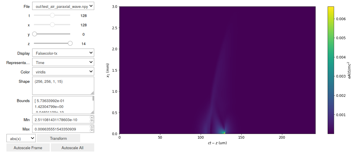
Fig. 3 — Interactive viewer with results from paraxial/air-fil.py example.