Reference
Module dispersion
Dispersion objects are used to specify a dispersion relation inside a volume object, or on either side of a surface object. The simplest way to use the dispersion module is to reference predefined materials. The available materials are listed in the following example:
mks_length = 0.8e-6/(2*np.pi)
air1 = dispersion.SimpleAir(mks_length)
air2 = dispersion.DryAir(mks_length)
air3 = dispersion.HumidAir(mks_length,0.4)
water = dispersion.LiquidWater(mks_length)
glass = dispersion.BK7(mks_length)
sodium_chloride = dispersion.NaCl(mks_length)
potassium_chloride = dispersion.KCl(mks_length)
zinc_selenide = dispersion.ZnSe(mks_length)
germanium = dispersion.Ge(mks_length)
It is simple to add a new medium to SeaRay if the dispersion relation can be put in Sellmeier form. To do so derive the new object from sellmeier_medium and provide the arrays of coefficients. See, e.g., the BK7 object for an example. You can also create a Sellmeier medium on the fly.
Required Methods
For dispersion that cannot be put in Sellmeier form you have to provide the following low level methods:
- dispersion.chi(w)
Calculate the susceptibility at a given frequency or set of frequenices. For compressible media, the susceptibility is given at a specific reference density. Dispersion objects are allowed to return either real or complex suceptibility, so higher level objects must be designed to handle either case.
- Parameters:
w (double) – the frequency or array frequencies to evaluate
- Returns:
susceptibility or array of susceptibilities corresponding to
w
- dispersion.Dxk(dens)
Creates a string containing OpenCL code that computes the local dispersion function

for use in ray tracing through non uniform media (this is the ray Hamiltonian, up to a parameterization).
- Parameters:
dens (str) – this string must contain an OpenCL function call that retrieves the density relative to the reference density.
- Returns:
String containing OpenCL code that computes the dispersion function
- dispersion.vg(xp)
Retrieve the group velocity for rays with phase space data xp. Must be written to accept variable number of dimensions (use ellipsis notation).
- Parameters:
xp (numpy.array) – The phase space data of the rays with shape (…,8)
- Returns:
the group velocity of the rays with shape (…,4)
Dispersion Classes
- class dispersion.sellmeier_medium(mks_length, A, L)
Dispersion object supporting susceptibility in the form:
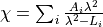
- __init__(mks_length, A, L)
Construct the dispersion object.
- Parameters:
mks_length (float) – the simulation unit of length in meters
A (numpy.array) – dimensionless coefficients in sum
L (numpy.array) – terms in sum with dimension of microns^2
Example:
x1 = 0.8e-6/(2*np.pi)
A = np.array([0.0])
L = np.array([0.0])
vacuum = dispersion.sellmeier_medium(x1,A,L)
- class dispersion.sellmeier_medium_alt1(mks_length, B, C)
Dispersion object supporting susceptibility in the form:
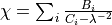
- __init__(mks_length, B, C)
Construct the dispersion object.
- Parameters:
mks_length (float) – the simulation unit of length in meters
B (numpy.array) – terms in sum with dimension of microns^-2
C (numpy.array) – terms in sum with dimension of microns^-2
Example:
x1 = 0.8e-6/(2*np.pi)
B = np.array([0.0])
C = np.array([0.0])
vacuum = dispersion.sellmeier_medium_alt1(x1,B,C)
- class dispersion.sellmeier_medium_alt2(mks_length, Nr, Ar, lr, rel_linewidth)
Dispersion object supporting susceptibility in the form:
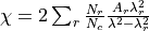 .
.This is a generalization of Eq. 4 from A.A. Voronin & A.M. Zheltikov, Nat. Sci. Rep. DOI:10.1038/srep46111. N.b. factor of 2 converting from index perturbation to susceptibility is appropriate only for tenuous media.
- __init__(mks_length, Nr, Ar, lr, rel_linewidth)
Construct the dispersion object.
- Parameters:
mks_length (float) – the simulation unit of length in meters
Nr (numpy.array) – terms in sum with dimension of cm^-3
Ar (numpy.array) – terms in sum, dimensionless
lr (numpy.array) – terms in sum with dimensions of nm
rel_linewidth (numpy.array) – relative linewidth of effective transitions, can be single value or an array.
Module surface
SeaRay surfaces are the fundamental object governing ray propagation.
Surfaces can reflect or refract rays, and collect field distributions.
They also serve as a boundary between different propagation models.
An optical medium is localized by enclosing it in a set of surfaces to form a volume.
All input dictionaries for surfaces have the following in common:
dispersion beneathmeans dispersion relation on negative z-side of surface.dispersion abovemeans dispersion relation on positive z-side of surface.originis the location of a reference point which differs by type of surface.euler anglesrotates the surface from the default orientation.
Applicable to all surfaces:
The default orientation is always such that a typical surface normal is in the positive z-direction.
Beneath the surface means negative z-side.
Above the surface means positive z-side.
If the surface bounds a volume, it should be oriented so that beneath resolves to inside and above resolves to outside.
A corollary to the above is that the normals point outward with respect to a volume.
Typical member functions assume arguments are given in local frame, i.e., the frame of the default orientation and position.
- class surface.AnalyticalMask(name)
Apply a spatial transfer function.
- Deflect(xp, eikonal, vg, vol: base_volume_interface | None)
The main SeaRay function handling reflection and refraction. Called from within Propagate(). Updates both the momentum and polarization.
- class surface.AsphericCap(name)
Positive radius has concavity in +z direction, parallel to normals
- class surface.BeamProfiler(name)
- Propagate(xp, eikonal, vg, orb={'idx': 0})
The main function to propagate ray bundles through the surface. Rays are left slightly downstream of the surface.
- class surface.CylindricalProfiler(name)
Place surface in an eikonal plane. Set “distance to caustic” to the distance from the eikonal plane to the center of the wave zone
- class surface.EikonalProfiler(name)
- class surface.Filter(name)
Apply a spectral transfer function.
- Deflect(xp, eikonal, vg, vol: base_volume_interface | None)
The main SeaRay function handling reflection and refraction. Called from within Propagate(). Updates both the momentum and polarization.
- class surface.FullWaveProfiler(name)
Place surface in an eikonal plane. Set “distance to caustic” to the distance from the eikonal plane to the center of the wave zone
- class surface.Grating(name)
- GetNormals(xp)
Premise is to select an effective normal based on ray frequency. Then the base_surface Deflect function can be re-used.
- class surface.IdealCompressor(name)
- Deflect(xp, eikonal, vg, vol: base_volume_interface | None)
The main SeaRay function handling reflection and refraction. Called from within Propagate(). Updates both the momentum and polarization.
- class surface.IdealHarmonicGenerator(name)
Move energy from w to 2w. Amplitude is exchanged between existing ray frequencies. We are following a protocol of never altering any ray frequency. The band refers to the band defining the pulse centered at the fundamental.
- Deflect(xp, eikonal, vg, vol: base_volume_interface | None)
The main SeaRay function handling reflection and refraction. Called from within Propagate(). Updates both the momentum and polarization.
- class surface.IdealLens(name)
The ideal lens will focus collimated rays to a perfect point. It will also adjust the phase to preserve pulse duration, just as a parabolic mirror would do.
- Deflect(xp, eikonal, vg, vol: base_volume_interface | None)
The main SeaRay function handling reflection and refraction. Called from within Propagate(). Updates both the momentum and polarization.
- class surface.LevelMap(name)
- class surface.NoiseMask(name)
- Deflect(xp, eikonal, vg, vol: base_volume_interface | None)
The main SeaRay function handling reflection and refraction. Called from within Propagate(). Updates both the momentum and polarization.
- class surface.Paraboloid(name)
Default position: paraboloid focus is at origin Default orientation: paraboloid vertex is at -f Acceptance angle defines angle between focused marginal ray and z-axis
- ClipImpact(xp)
- Returns:
booleans of shape (bundles,rays) where true indicates a clipped ray
- Return type:
numpy.array
- class surface.SphericalCap(name)
Default position: center of sphere is at +Rs Default orientation: cap centroid is at origin
- ClipImpact(xp)
- Returns:
booleans of shape (bundles,rays) where true indicates a clipped ray
- Return type:
numpy.array
- class surface.base_surface(name)
Base class for deriving surfaces.
- ClipImpact(xp)
- Returns:
booleans of shape (bundles,rays) where true indicates a clipped ray
- Return type:
numpy.array
- Deflect(xp, eikonal, vg, vol: base_volume_interface | None)
The main SeaRay function handling reflection and refraction. Called from within Propagate(). Updates both the momentum and polarization.
- Detect(xp, vg)
Determine which bundles should interact with the surface.
- Returns:
time of ray impact, indices of impacting bundles
- Return type:
numpy.array, numpy.array, numpy.array
- GetRelDensity(xp, vol: base_volume_interface | None)
Get the density at the ray position from the enclosed volume object
- PositionGlobalToLocal(xp)
Transform position vectors only
- PositionLocalToGlobal(xp)
Transform position vectors only
- Propagate(xp, eikonal, vg, orb={'idx': 0}, vol: base_volume_interface | None = None)
The main function to propagate ray bundles through the surface. Rays are left slightly downstream of the surface.
- RaysGlobalToLocal(xp, eikonal, vg)
Transform all ray data from the global system to the local system associated with this surface.
- Parameters:
xp (numpy.array) – phase space data
eikonal (numpy.array) – eikonal amplitude and phase
- RaysLocalToGlobal(xp, eikonal, vg)
Transform all ray data from the system associated with this surface to the global system.
- Parameters:
xp (numpy.array) – phase space data
eikonal (numpy.array) – eikonal amplitude and phase
- SelectBand(xp)
Get an array of bundle indices in the passband
- UpdateOrbits(xp, eikonal, orb)
Append a time level to the orbits data and advance the index.
- class surface.cylindrical_shell(name)
Default position : cylinder centered at origin Default orientation : cylinder axis is z-axis Dispersion beneath means inside the cylinder, above is outside
- ClipImpact(xp)
- Returns:
booleans of shape (bundles,rays) where true indicates a clipped ray
- Return type:
numpy.array
- class surface.disc(name)
- ClipImpact(xp)
- Returns:
booleans of shape (bundles,rays) where true indicates a clipped ray
- Return type:
numpy.array
- class surface.quadratic(name)
- Detect(xp0, vg)
Determine which bundles should interact with the surface.
- Returns:
time of ray impact, indices of impacting bundles
- Return type:
numpy.array, numpy.array, numpy.array
- class surface.rectangle(name)
- ClipImpact(xp)
- Returns:
booleans of shape (bundles,rays) where true indicates a clipped ray
- Return type:
numpy.array
- class surface.surface_mesh(name)
- Detect(xp, vg)
Performs an efficient search for the target simplex. Assumes linear trajectory cannot cross more than one simplex.
- Propagate(xp, eikonal, vg, orb={'idx': 0}, vol: base_volume_interface | None = None)
Propagate rays through a surface mesh. The medium on either side must be uniform.
- class surface.triangle(a, b, c, n0, n1, n2, disp1, disp2, bandpass=(0.0, 100.0))
Building block class, does not respond to input file dictionaries. Meant to be used as an element in surface_mesh class.
- ClipImpact(xp)
- Returns:
booleans of shape (bundles,rays) where true indicates a clipped ray
- Return type:
numpy.array
Module volume
All input dictionaries for volumes have the following in common:
dispersion insidemeans dispersion inside the volume.dispersion outsidemeans dispersion outside the volume.originis the location of a reference point which differs by type of volume.euler anglesrotates the volume from the default orientation.
This module uses multiple inheritance resulting in a diamond structure. All volumes inherit from base_volume.
This branches into some objects that describe a region, and others that describe a nonuniformity inside the region.
Nonuniform volumes are derived from both, hence the diamond structure.
It is important to use the super() function in the initialization chain.
There is a concept of “reference density” and “relative density” herein. The reference density is a density whereat optical parameters are specified, e.g., dispersion parameters. The relative density is the ratio of density to reference density. A possible source of confusion is that the reference density is itself normalized.
- class volume.AnalyticBox(name)
Fill a box with an analytical density profile. See also AnalyticDensity class.
- class volume.AnalyticCylinder(name)
Fill a cylinder with an analytical density profile. See also AnalyticDensity class.
- class volume.AnalyticDensity(name)
Base class used to create an analytical density profile. Input dictionary key “density function” is a string containing a CL expression which may depend on x and r2. Here x is a double4, x.s1 = x, x.s2 = y, x.s3 = z, and r2 = x**2 + y**2 Input dictionary key “density lambda” is a Python lambda function of (x,y,z,r2). Here the arguments are numpy arrays with shape (bundles,rays), and the return value must have the same shape.
- GetRelDensity(xp)
Density relative to reference density
- class volume.AsphericLens(name)
Curved beneath, planar above. curvature radius is signed. Positive sign is convex, negative is concave. The thickness is measured along central axis of lens. The extremities on axis are equidistant from the origin
- class volume.AxisymmetricTestGrid(name)
- class volume.Box(name)
- class volume.Cylinder(name)
- class volume.PellinBroca(name)
Pellin-Broca Prism. Local origin is the pivot point, which is on side C. The
sizetuple is given as (A,h,B) where h is the height, A is the input side length, and B is the output side length. Sides C and D are inferred from theangleparameter (refraction angle through A, also angle AD), and the requirement that input and output beams make a 90 degree angle. Side C is the reflector:B ------------ | | x | | ^ A | * C | | | | | | -------> z | ---- ---- D
- class volume.PellinBroca2(name)
Alternate Pellin-Broca Prism. The pivot point, on side D, is placed at the origin. The
sizetuple is given as (A,h,B) where h is the height, A is the input side length, and B is the output side length. Sides C and D are inferred from theangleparameter (refraction angle through A, also angle AD-pi/4), and the requirement that input and output beams make a 90 degree angle. Side D is the reflector:B --------------- | | x | | C ^ A | ------ | | ---*- | ---- D ------> z
- class volume.Prism(name)
Isoceles prism. Dispersion is in local xz plane. Base is in the plane x = -size[0]/2.
- class volume.RetroPrism(name)
Same as Prism but assumes TIR on one surface.
- class volume.SphericalLens(name)
rcurv beneath and above are signed radii of curvature. Positive radius means concavity faces +z. The thickness is measured along central axis of lens. The extremities on axis are equidistant from the origin. Surfaces need to be carefully oriented so that normals are outward.
- class volume.TestGrid(name)
- class volume.base_volume(name)
The base_volume is an abstract class which takes care of rays entering and exiting an arbitrary collection of surfaces that form a closed region. Volumes filled uniformly can be derived simply by creating the surface list in
self.Initialize.- GetRelDensity(xp)
Density relative to reference density
- class volume.grid_volume(name)
- class volume.nonuniform_volume(name)
Module: ray_kernel
This module is the primary computational engine for ray tracing with eikonal field data.
- ray_kernel.ConfigureRayOrientation(xp, eikonal, vg, origin, euler)
Rotate all rays using the provided Euler angles and move to origin.
- ray_kernel.GetMicroAction(xp, eik, vg)
Numerical accuracy metric, should be conserved.
- ray_kernel.GetTransversality(xp, eik)
Numerical accuracy metric, should be unity in isotropic media.
- ray_kernel.PulseSpectrum(xp, N, box, pulse_length, w0)
Weight the rays based their frequency. Assume transform limited pulse. Spectral amplitude is matched with time domain amplitude by performing a test FFT. If the lower frequency bound is zero, real carrier resolved fields are used.
- Parameters:
xp (numpy.ndarray) – Ray phase space, primary ray frequency must be loaded
N (tuple) – The first element is the number of frequency nodes
box (tuple) – The first two elements are the frequency bounds
pulse_length – The Gaussian pulse width (1/e amplitude)
w0 – The central frequency of the wave
- Returns:
weight factors with shape (bundles,)
- ray_kernel.gather(cl, xp, dens)
Return density at location of each ray (primary + satellites).
- ray_kernel.init(source)
Use source dictionary from input file to create initial ray distribution. Vacuum is assumed as the initial environment. Rays are packed in bundles of 4. If there are Nb bundles, there are Nb*4 rays.
- Returns:
xp,eikonal,vg
- Return type:
numpy.ndarray((Nb,4,8)),numpy.ndarray((Nb,4)),numpy.ndarray((Nb,4,4))
The 8 elements of xp are x0,x1,x2,x3,k0,k1,k2,k3. The 4 elements of eikonal are phase,ax,ay,az. The 4 elements of vg are 1,vx,vy,vz.
- ray_kernel.load_rays_eik(xp, eikonal, vg, N, box, waves)
Load momentum, amplitude, and phase using a paraxial superposition. The superposition waves should have minimal overlap in ray space (w,x,y). It is assumed we are in a basis where the waist is at the origin and the wavevector is oriented in the +z direction.
- ray_kernel.load_rays_xw(xp, bundle_radius, N, box, loading_coordinates)
Load the rays in the z=0 plane in a regular pattern. Momentum, amplitude, and phase are left undefined.
- ray_kernel.track(cl, xp, eikonal, vol_dict, orb)
Move rays through a volume using an analytical density function.
- Parameters:
cl (cl_refs) – OpenCL reference class
xp (np.ndarray) – phase space for all rays, kernel must handle outliers
eikonal (np.ndarray) – eikonal data for all rays, kernel must handle outliers
vol_dict (dict) – volume dictionary input object
orb (dict) – dictionary of orbit information
- ray_kernel.track_RIC(cl, xp, eikonal, dens, vol_dict, orb)
Move rays through a volume using ray-in-cell method.
- Parameters:
cl (cl_refs) – OpenCL reference class
xp (np.ndarray) – phase space for all rays, kernel must handle outliers
eikonal (np.ndarray) – eikonal data for all rays, kernel must handle outliers
dens (np.ndarray) – the density data
vol_dict (dict) – volume dictionary input object
orb (dict) – dictionary of orbit information
Module: paraxial_kernel
This module is the primary computational engine for advancing paraxial wave equations. The call stack is as follows:
track is called externally
track repeatedly calls propagator to advance to the end of the volume
propagator repeatedly calls load_source and RK4 functions to advance to the next diagnostic plane
load_source has these steps
propagate linearly
transform (kx,ky) -> (x,y)
call update_current
transform (x,y) -> (kx,ky)
estimate step size if requested
- class paraxial_kernel.Material(queue, ctool: ~caustic_tools.CausticTool, N: tuple, coords: str, vol: ~base.base_volume_interface, chi: <MagicMock id='140590727740864'>, chi3: <MagicMock id='140590727842928'>, nref: <MagicMock id='140590728058032'>, w0: <MagicMock id='140590728065376'>, ng: <MagicMock id='140590727504720'>, n0: <MagicMock id='140590727816880'>)
This class manages host and device storage describing the material’s density and susceptibility. It also computes the generator of linear axial translations, kz.
- class paraxial_kernel.Source(queue, a: <MagicMock id='140590728213408'>, w: <MagicMock id='140590728205680'>, zi: <MagicMock id='140590728269200'>, L: <MagicMock id='140590727826112'>)
This class gathers references to host and device storage that are used during the ODE integrator right-hand-side evaluation.
- paraxial_kernel.finish(cl: ~init.cl_refs, T: ~grid_tools.TransverseModeTool, src: ~paraxial_kernel.Source, mat: ~paraxial_kernel.Material, ionizer: ~ionization.Ionizer, rotator: ~rotations.Rotator, zf: <MagicMock id='140590727722608'>) tuple[<MagicMock id='140590728128080'>, <MagicMock id='140590728125296'>, <MagicMock id='140590727455280'>, <MagicMock id='140590727457008'>]
Finalize data at the end of the iterations and retrieve.
- Parameters:
cl (cl_refs) – OpenCL reference bundle
T (TransverseModeTool) – used for transverse mode transformations
src (Source) – stores references to OpenCL buffers used in RHS evaluations
mat (Material) – stores references to OpenCL buffers used in Linear propagation
ionizer (Ionization) – class for encapsulating ionization models
rotator (Rotator) – class for encapsulating molecular rotations
zf (double) – global coordinate of the final position
- paraxial_kernel.load_source(z0: <MagicMock id='140590727833984'>, z: <MagicMock id='140590727716176'>, cl: ~init.cl_refs, T: ~grid_tools.TransverseModeTool, src: ~paraxial_kernel.Source, mat: ~paraxial_kernel.Material, ionizer: ~ionization.Ionizer, rotator: ~rotations.Rotator, return_dz=False)
We have an equation in the form dq/dz = S(z,q). This loads src.J_dev with S(z,q), using q = src.qw_dev
- Parameters:
z0 (double) – global coordinate of the start of the subcycle region
z (double) – local coordinate of evaluation point referenced to z0
cl (cl_refs) – OpenCL reference bundle
T (TransverseModeTool) – used for transverse mode transformations
src (Source) – stores references to OpenCL buffers used in RHS evaluations
mat (Material) – stores references to OpenCL buffers used in Linear propagation
ionizer (Ionization) – class for encapsulating ionization models
rotator (Rotator) – class for encapsulating molecular rotations
return_dz (bool) – if true return the step size estimate
- paraxial_kernel.propagator(cl: ~init.cl_refs, ctool: ~caustic_tools.CausticTool, a: <MagicMock id='140590727607584'>, mat: ~paraxial_kernel.Material, ionizer: ~ionization.Ionizer, rotator: ~rotations.Rotator, subcycles: int, zi: <MagicMock id='140590727794208'>, zf: <MagicMock id='140590727801984'>)
Advance a[w,x,y] to a new z plane using paraxial wave equation. Works in either Cartesian or cylindrical geometry. If cylindrical, intepret x as radial and y as azimuthal. The RK4 stepper is advancing q(z;w,kx,ky) = exp(-i*kz*z)*a(z;w,kx,ky).
- Parameters:
cl (cl_refs) – OpenCL reference bundle
ctool (CausticTool) – contains grid info and transverse mode tool
a (numpy.array) – the vector potential in representation (w,x,y) as type complex
mat (Material) – stores references to OpenCL buffers used in Linear propagation
ionizer (Ionization) – class for encapsulating ionization models
rotator (Rotator) – class for encapsulating molecular rotations
subcycles (int) – number of density evaluations along the path
zi (double) – initial z position
zf (double) – final z position
- paraxial_kernel.track(cl, xp, eikonal, vg, vol_dict: dict)
Propagate paraxial waves using eikonal data as a boundary condition. The volume must be oriented so the polarization axis is x (linear polarization only).
- Parameters:
xp (numpy.array) – ray phase space with shape (bundles,rays,8)
eikonal (numpy.array) – ray eikonal data with shape (bundles,4)
vg (numpy.array) – ray group velocity with shape (bundles,rays,4)
vol_dict (dictionary) – input file dictionary for the volume
- paraxial_kernel.update_current(cl: cl_refs, src: Source, mat: Material, ionizer: Ionizer, rotator: Rotator)
Get current density from A[w,x,y]
Module: uppe_kernel
This module is the primary computational engine for advancing unidirectional pulse propagation equations (UPPE). The call stack is as follows:
track is called externally
track repeatedly calls propagator to advance to the end of the volume
propagator advances to the next diagnostic plane by repeatedly calling
load_source
RK4 functions
condition_field
load_source has these steps
propagate linearly
transform (kx,ky) -> (x,y)
call update_current
transform (x,y) -> (kx,ky)
estimate step size if requested
- class uppe_kernel.Material(queue, ctool, N, coords, vol, chi, chi3, nref, vg)
This class manages host and device storage describing the material’s density and susceptibility. It also computes the generator of linear axial translations, kz.
- class uppe_kernel.Source(queue, a, w, zi, L, NL_band)
This class gathers references to host and device storage that are used during the ODE integrator right-hand-side evaluation.
- uppe_kernel.condition_field(cl, src)
Impose filters or other conditions on field
- uppe_kernel.finish(cl, T, src, mat, ionizer, rotator, zf)
Finalize data at the end of the iterations and retrieve.
- Parameters:
cl (cl_refs) – OpenCL reference bundle
T (TransverseModeTool) – used for transverse mode transformations
src (source_cluster) – stores references to OpenCL buffers
mat (Material) – stores references to OpenCL buffers used in Linear propagation
ionizer (Ionization) – class for encapsulating ionization models
rotator (Rotator) – class for encapsulating molecular rotations
zf (double) – global coordinate of the final position
- uppe_kernel.load_source(z0, z, cl, T, src, mat, ionizer, rotator, return_dz=False, dzmin=1.0)
We have an equation in the form dq/dz = S(z,q). This loads src.Jw_dev with S(z,q), using src.qw_dev
- Parameters:
z0 (double) – global coordinate of the start of the subcycle region
z (double) – local coordinate of evaluation point referenced to z0
cl (cl_refs) – OpenCL reference bundle
T (TransverseModeTool) – used for transverse mode transformations
src (Source) – stores references to OpenCL buffers used in RHS evaluations
mat (Material) – stores references to OpenCL buffers used in Linear propagation
ionizer (Ionization) – class for encapsulating ionization models
rotator (Rotator) – class for encapsulating molecular rotations
return_dz (bool) – return step size estimate if true
- uppe_kernel.propagator(cl, ctool, vg, a, mat, ionizer, rotator, NL_band, subcycles, zi, zf, dzmin)
Advance a[mu,w,x,y] to a new z plane using UPPE method; mu = 4-vector index. Works in either Cartesian or cylindrical geometry. If cylindrical, intepret x as radial and y as azimuthal. The RK4 stepper is advancing q(z;w,kx,ky) = exp(-i*(kz+kg)*z)*a(z;w,kx,ky). In the time domain the kg(w) wavevector results in a(t-vg*z,x,y), i.e., gives us the pulse frame.
- Parameters:
cl (cl_refs) – OpenCL reference bundle
ctool (CausticTool) – contains grid info and transverse mode tool
vg (double) – the window velocity
a (numpy.array) – the vector potential in representation (mu,w,x,y) as type complex
mat (Material) – stores references to OpenCL buffers used in Linear propagation
ionizer (Ionization) – class for encapsulating ionization models
rotator (Rotator) – class for encapsulating molecular rotations
NL_band (tuple) – filter applied to nonlinear source terms
subcycles (int) – number of density evaluations along the path
zi (double) – initial z position
zf (double) – final z position
dzmin (doulbe) – minimum step size
- uppe_kernel.track(cl, xp, eikonal, vg, vol_dict)
Propagate unidirectional fully dispersive waves using eikonal data as a boundary condition. The volume must be oriented so the polarization axis is x (linear polarization only).
- Parameters:
xp (numpy.array) – ray phase space with shape (bundles,rays,8)
eikonal (numpy.array) – ray eikonal data with shape (bundles,4)
vg (numpy.array) – ray group velocity with shape (bundles,rays,4)
vol_dict (dictionary) – input file dictionary for the volume
- uppe_kernel.update_current(cl, src, mat, ionizer: Ionizer, rotator: Rotator)
Get current density from A[w,x,y]
Module: grid_tools
Tools for transforming between structured and unstructured grids, and spectral analysis. Ray data can be viewed as known on the nodes of an unstructured grid. Our notion of a structured grid is that the data is known at the cell center. The set of cell centers are the nodes. The nodes are separated by cell walls. Plotting voxels can be considered visualizations of a cell.
- grid_tools.CylGridFromInterpolation(w, x, y, vals, wn=1, xn=100, yn=100, fill=0.0)
Special treatment for points that tend to lie on cylindrical nodes. Frequency and azimuth are binned, radial data is interpolated. Fill value for r<min(r) is val(min(r)). w,x,y,vals are the irregular data points, where x,y are interpreted as rho,phi. (ray coordinate system is transformed externally) wn,xn,yn are regular arrays of nodes, or numbers of nodes. If numbers are given, the node boundaries are obtained from the points.
- grid_tools.DataFromGrid(w, x, y, wn, xn, yn, the_data)
Form irregular data from a regular grid. OK if yn.shape[0]=1. w,x,y are the coordinates of the irregular data points. Irregular points can be slightly outside the grid (extrapolation is used). wn,xn,yn are arrays of nodes which must be regularly spaced. the_data contains values on the regular grid with shape (w,x,y). Any coordinate transformations must happen externally.
- class grid_tools.FourierTransformTool(N, dq, cl)
Transform Cartesian components to plane wave basis
- grid_tools.GridFromBinning(x, y, z, xn=100, yn=100)
x,y,z are the data points. xn,yn are arrays of nodes, or numbers of nodes. If numbers are given, the node boundaries are obtained from the points.
- grid_tools.GridFromInterpolation(w, x, y, vals, wn=1, xn=100, yn=100, fill=0.0)
w,x,y,vals are the irregular data points. wn,xn,yn are regular arrays of nodes, or numbers of nodes. If numbers are given, the node boundaries are obtained from the points.
- class grid_tools.HankelTransformTool(Nr, dr, mmax, cl, Nk)
Transform Cartesian components to Bessel beam basis.
- class grid_tools.TransverseModeTool(N, dq, cl)
Base class for transformation of Cartesian components to another spatial basis
- Parameters:
N (4-tuple) – nodes along each dimension (0 and 3 are not used)
dq (4-tuple) – node separation along each dimension (must be uniform)
- grid_tools.cell_centers(wall_pos_low, wall_pos_high, cells_between)
Generate nodes between two cell wall positions. Number of nodes between the two walls must be given.
- grid_tools.cell_walls(node_low, node_high, nodes_between, default_voxel_width=1000.0)
Generate cell walls bracketing two nodes. Number of nodes between the walls must be given.
- grid_tools.cyclic_center_and_width(node_low, node_high)
Return the center node and wall-to-wall width of a cyclic set of nodes. Once cyclic nodes are generated the high node is lost. This function helps us remember not to use the generated nodes to find the center. See also cyclic_nodes(…) below.
- grid_tools.cyclic_nodes(node_low, node_high, num_nodes)
Generate nodes suitable for periodic functions. The requested low node is included, the high node is excluded. The low and high nodes should resolve to the same point, e.g. 0 and 2*pi. Frequency nodes are arranged in unrolled FFT fashion, e.g., [+-2,-1,0,1].