Running on the Desktop

Caution

This document assumes you have followed the installation instructions precisely. Once installed, running SeaRay should be the same for any UNIX-based desktop system.

Tip

You can issue UNIX like commands in Windows via the PowerShell. Otherwise, use the Anaconda prompt and replace the forward slash with the backslash in directory paths.

OpenCL Background

In order to run SeaRay, it is useful to understand a little about OpenCL. SeaRay uses a Python wrapper for OpenCL, called PyOpenCL, to accelerate certain computations. OpenCL is designed to interface with arbitrary computing devices, especially multi-core CPU and general purpose GPU (GPGPU) devices. For this reason the user is invited to specify a device to use for these accelerations. This specification is optional, but if SeaRay tries to choose a device on its own, and that device turns out not to be appropriate, the run may fail. The two failure modes most likely are (i) not enough memory on the device, and (ii) not enough floating point precision on the device.

Running a Ray Example

1. Activate your virtual environment (see Generic SeaRay Installation)
2. Pick some example from raysroot/examples/eikonal/.
3. For definiteness, let us use raysroot/examples/eikonal/parabola.py
4. Open a terminal window and navigate to raysroot
5. python rays.py list
6. The above command lists the hardware acceleration platforms and devices available on your system. A device may be available only within a given platform. If there is more than one platform, choose the one you would like to use, and pick out some unique part of its name, such as cuda. Case does not matter. Similarly, if there is more than one device, choose some unique part of its name, such as titan
7. python rays.py run file=examples/eikonal/parabola.py platform=cuda device=titan
8. This copies the parabola.py example file to the raysroot directory as inputs.py and runs the calculation. If you do not specify a file, SeaRay will use whatever inputs.py is in raysroot. It is best practice to never directly edit inputs.py.
9. When the run is finished, you should have several output files in raysroot/out. The output files are simply pickled numpy arrays.
10. Let us plot the results using the SeaRay plotter. The plotter is not interactive, but allows for a fairly high degree of control using command line options. You can get a help screen by executing python ray_plotter.py with no arguments.
11. python ray_plotter.py out/test o3d
12. You should see a 3D rendering of the ray orbits reflecting off an off-axis parabola, as in Fig. 1 below (assuming matplotlib environment). When you are done looking close the plot window.
13. python ray_plotter.py out/test det=1,2/0,0/0.1
14. This should produce an image of the radiation intensity at the focal point, as in Fig. 2 below.

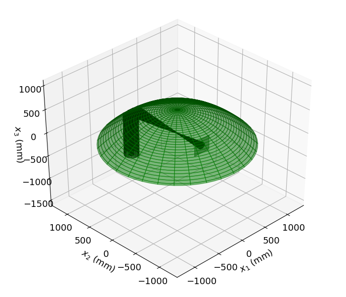
Fig. 1 — ray orbits from parabolic mirror example

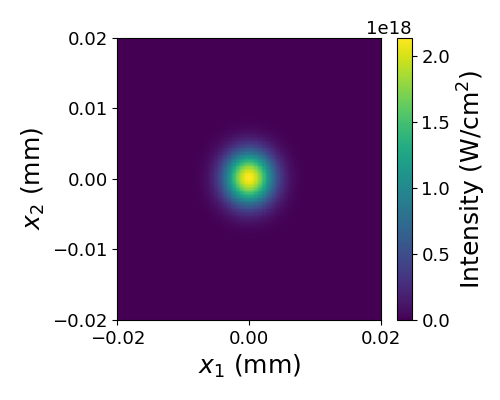
Fig. 2 — Intensity at best focus

Running a Wave Example

1. Activate your virtual environment (see Generic SeaRay Installation)
2. Run the example case raysroot/examples/paraxial/air-fil.py following the same general procedure as above.
3. Wave runs typically take longer, although this one is fairly quick. You should see some text based progress indicators as the wave propagation is calculated. The time stepper is adaptive, so varying amounts of work may be done between diagnostic planes.
4. At present you must use the Jupyter-based interactive viewer to plot the results. For the following Jupyter and ipympl must be installed in your environment.
5. jupyter notebook
6. When the Jupyter home page comes up select ray_viewer.ipynb.
7. For this example you should not need to change the source code. Generally, if output files are saved under a different location you have to change the value of base_diagnostic. Note also that as of this writing, the normalizing length is hard coded in the notebook.
8. Run the notebook (select Run All from the Cell menu). Advance the z-slider to observe the pulse evolution.

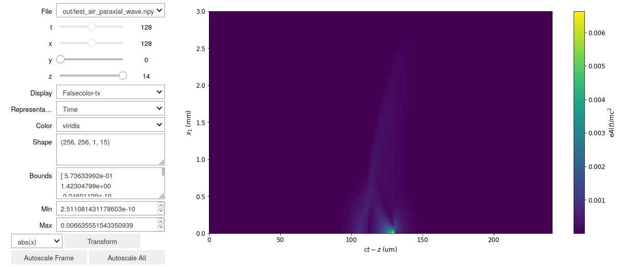
Fig. 3 — Interactive viewer with results from paraxial/air-fil.py example.